Kernel Mixture Networks

On a regular basis I feel like default mean regression is not enough for use cases I am working on. Modeling the uncertainty of reality and of the model itself can add a lot value, in particular for scenarios where decisions have to be made based on the output of a predictive model. By predicting full probability distributions conditioned on your input (what will out output look like, given this specific input) we get a lot more information if done properly. If necessary, this distribution can always be collapsed into a mean again.

Common use cases are:

• Monte Carlo sampling from (conditional) distribution
• Exploitation versus exploration dilemma in reinforcement learning
• Quantile regression without specifically training on one quantile
• Reversed quantile information, estimating the probability that the output will be lower or higher than a non-predetermined $y$
• Having non-linear costs after the output that require more knowledge than the expected value

In this blog post I will first look at common approaches to unconditional density estimation and subsequently extend these approaches to conditional density estimations. Next, I will examine a freshly released paper called The Kernel Mixture Network: A Nonparametric Method for Conditional Density Estimation of Continuous Random Variables where the authors use a new combination to tackle this problem. In addition to going through a Python implementation by my colleague Alexander Backus and myself, we will also consider some potential extensions of this paper.

Unconditional density estimation

With unconditional density estimation we are interested in estimating $p(\mathbf{x})$, a (joint) probability distribution over n dimensions. In this section we will look at a set of points generated by a standard 1-dimensional Gaussian with $\mu=0$ and $\sigma=1$, see how the different estimations are affected by increasing sample sizes and what the downsides are of each method, before extending these to conditional density estimation techniques.

Histogram

A histogram discretizes your input dimension by counting the number of observations that fall within each predefined range. After normalizing the counts so that the surfaces of the bars with the bin widths and the normalized count as height sum to 1. Setting the bin width is a parameter of your distribution, as well as determining where the bins start and finish. There are numerous methods for this which we will not go into, but I would like to show the effect of sample size on the histogram:

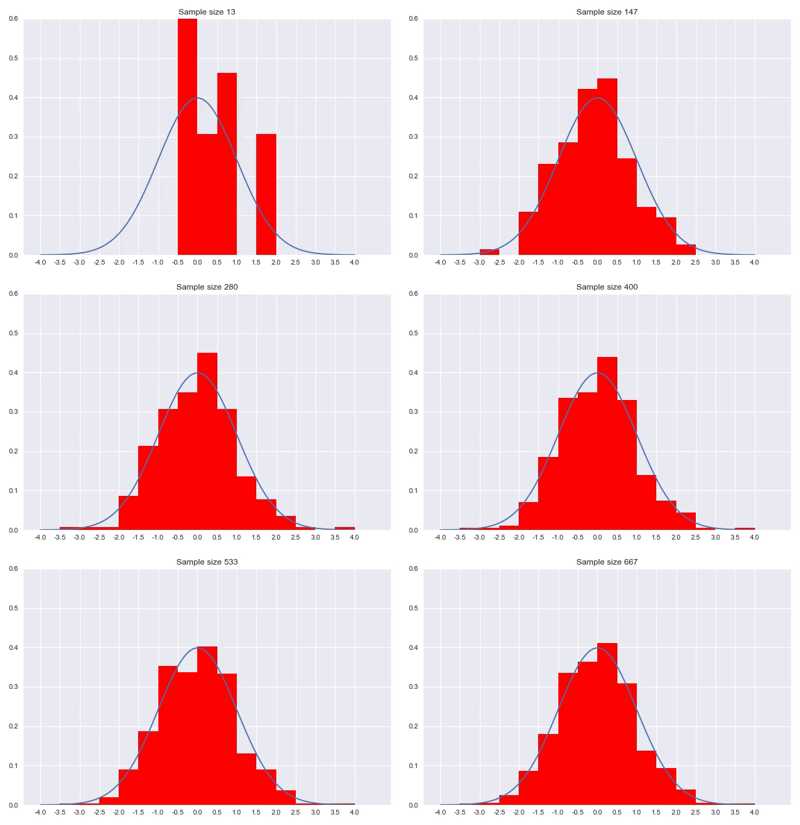
As we can see in the animation, it takes a considerable number of samples to get close to the true distribution. In addition since we discretized our data, we can never get really close without increasing to a high amount of bins. A very small bin width will increase the variance of the count and overfits on your data, while a bin width that is too big will obfuscate relevant information by averaging out details. An advantage of histograms is that the procedure makes few assumptions with regards to the shape of distribution that generated your data, plus it is a very intuitive way of visualizing a distribution. That said, getting the bin width right is tricky, using it to approximate a distribution means the range is bounded by the beginning and end of your bins and points near the borders of the bins might be closer to points in the neighboring bin than any point in it’s own bin.

The probability density of a histogram distribution can described by:

Where $\mathfrak{U}_j(x)$ is the height of bin $j$ if $x$ falls within bin $j$, otherwise 0.

Fitting parameterized distributions

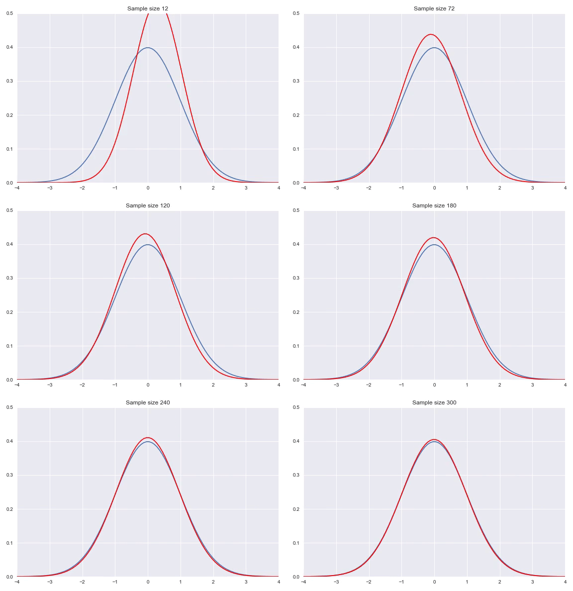
Instead of using a non-parametric approach like histograms or kernel density estimation we can also use parametric distributions where we estimate the parameters to fit the assumed distribution. If the family of distributions fits the data well we can get very nice fits with relatively little amount of data, however, if the family does not fit the generating distribution properly you will get poor results. Some standard distributions, for example Gaussians are easy to fit by just looking at some statistics of your data. In case of the Gaussian the mean $\hat{\mu} = \overline{X} = \frac{\sum_{i=1}^nx_i}{n}$ and $\hat{\sigma}^2=\frac{\sum_{i=1}^n(x_i-\overline{X})^2}{n-1}$ will produce the most likely Gaussian that generated your data. In more complicated distributions you will need to use some form of iterative optimization, for instance using gradient descent on the likelihood function to fit your parameters. Below, I have illustrated a Gaussian fit on our data generated by a default Gaussian. Notice that this animation uses smaller sample sizes.

Combining different distributions by weighing them extends the space of distributions that we can describe quite substantially, while still keeping the amount of parameters within reason. Sampling from these so called mixtures is easy. We first sample from a discrete distribution that determines from which subdistribution we actually sample from. The full density is defined by:

Here, $\pi_j$ is the weight of subdistribution $j$, all $\pi_j\geq 0$ and $\sum_{j=1}^k\pi_j = 1$.

Kernel density estimation

An alternative non-parametric option is kernel density estimation. The core concept is that every observation in our data contributes to a small subdistribution in our full distribution. We do this by defining a distribution around each observation itself, using a kernel. A kernel is a function that is non-negative real-valued and in the case of non-parametric statistics preferably integrates to $1$ and is symmetric. These kernel functions usually represent some kind of similarity between two points in a space. The idea is to use every observation as a kernel center, because we have evidence that this point was generated by the distribution that we want to estimate. There are many types of kernels we can choose from, empirically it is not very important however. You do have to be careful that all your new observations will have a strictly positive likelihood like with the histogram, because we know the density has to be strictly positive, else we could not have observed the point. Regularly Gaussian kernels are used, these are defined as follows:

We define this kernel for every of our observations and weight them with a factor $\frac{1}{n}$, which means the sum of these weighted kernels integrate to $1$ again. This makes our estimated density function:

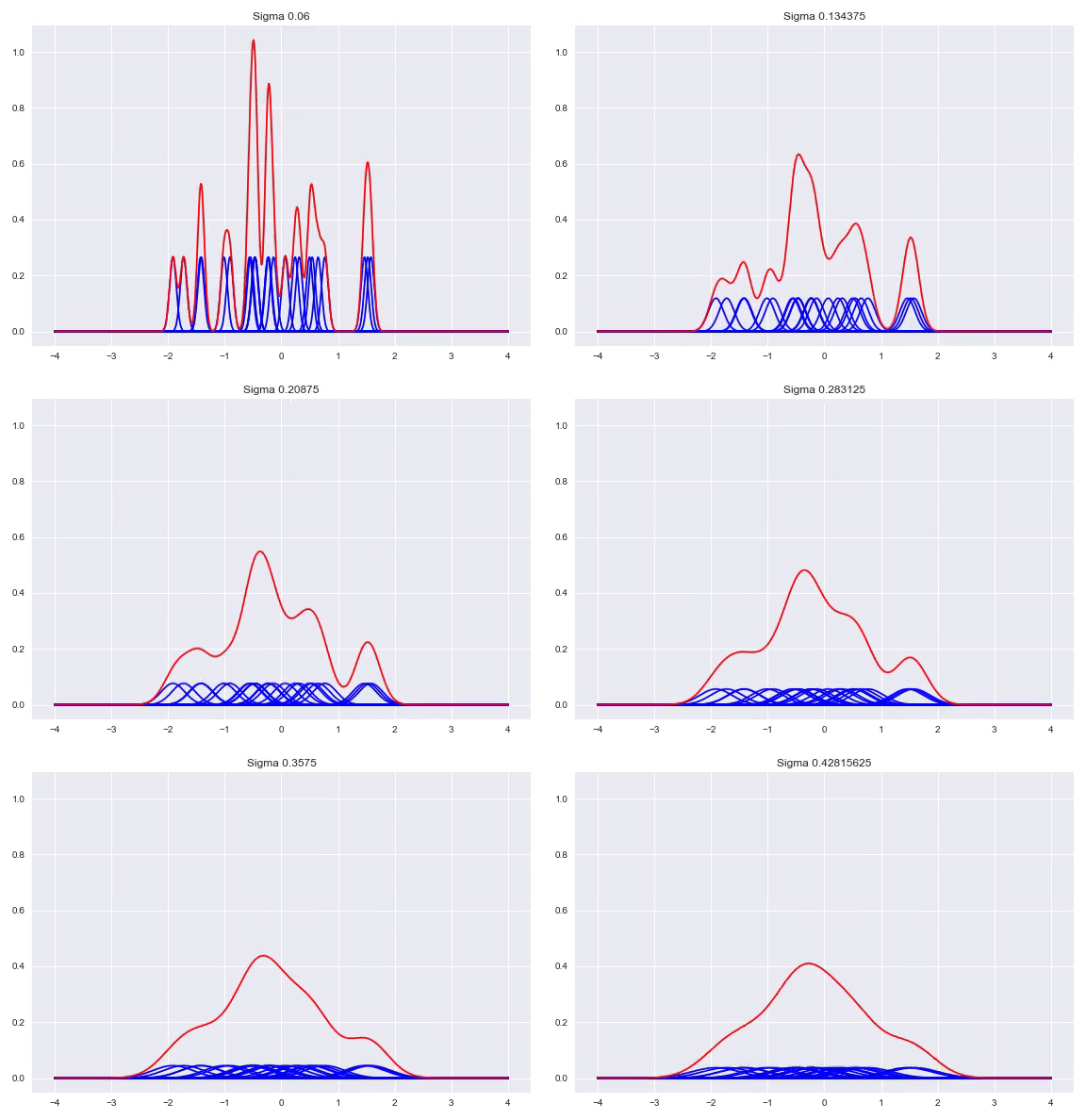
The $\sigma$ determines the bandwidth of the kernel, which heavily influences the shape of our distribution. While there are some heuristics to calculate a good bandwidth value, using a cross validation procedure with a number of bandwidths evaluated with the log likelihood is the preferred method. A bandwidth that is too small will generate a very wonky distribution while a bandwidth that is too larg will lose a lot of its nuance in a similar way as the histogram does with bins that are too wide. Here, we can see the effect of the bandwidth size on the shape of the distribution, from a sample size of 25:

Conditional density estimation

Previously, we consider the entire data set $X$ for densities. Instead, we are now going to look for cases where we want to estimate a probability distribution over $y$, given their corresponding $\mathbf{x}$. Training and evaluating of these models usually involves the likelihood of our model $m$ given our data $(\mathbf{x}, y)$. Note that this is equivalent to the density of our data given our model $m$. By looking at every observation and calculating the value of our density function for that $y$ given our model and the corresponding features $\mathbf{x}$, and then taking the product of each of these densities we arrive at the likelihood:

Due to numerical stability, the log likelihood is used, turning the product into a sum of logarithms, for optimization is the same, given that the log function is monotonicly increasing. By convention, loss functions are minimized with neural networks, this means we will negate it and call it the negative log-likelihood:

In case $ P(y_i \mid \mathbf{x_i}, m) $ is differentiable the negative log-likelihood is also differentiable, which means we can plug this into our favorite deep learning package and optimize our model directly, which is how the approaches we will discuss next work. The output layers that we will talk about in the rest of this post can be stacked on top of any normal layer in a neural network. For example, on top of a normal feed forward network but also on the hidden state of recurrent networks or after a convolutional layer.

Quantized softmax networks

With a quantized softmax network, we estimate the height of each bar in a normalized histogram. We can perform this estimation by chopping up the range of your output into n equally sized bins with a uniform density attached to each bin. The neural network will have n output nodes that have a softmax activation, to ensure that the output nodes sum to 1. Each output node represents the height of the corresponding bin. Given that the density integrated to 1 before weighing them, it still does because the bins are equal width and the weights still sum to 1. The density is now:

Here $z_j$ represents output node $j$ given our input $\mathbf{x}$ and our trained neural network parameters $W$. To train our network we will feed it pairs of samples and backpropagate our negative log-likelihood loss through the graph. Conceptually, the best the network can do is put all the weight on the bin that $y$ belongs to, which means it will adapt $W$ to increase the weight at the corresponding bin and decrease the weight at the other bins. This approach is very intuitive and effective. It is severely restrictive in the shape of the estimated distribution however, due to the discretization of the output space and that the network will $NaN$ out when you have a $y$ that is outside of your bins, due to a $\log(0)$ in your loss function. That said, adding more bins only costs $m$ parameters per extra bin where $m$ is the size of the layer before the output layer.

Mixture density networks

As seen before, we can fit parameterized distributions using gradient descent. However, instead of having these parameters fixed, we can also condition them on our input. This approach is similar to estimating the weight distribution over the bins in a quantized softmax network. In case of predicting a Gaussian distribution given our input $x$, we would have a neural network with two outputs, one with an identity activation to represent $\mu(x)$ and one that needs a monotonically increasing strictly positive activation for $\sigma(x)$, for example the exponential activation $e^x$ or a softplus activation $\ln{(1+e^x)}$. Now we can optimize our network by minimizing the negative log-likelihood of our training examples. A potential caveat arises when the model is too expressive and can heavily overfit by memorizing all the training samples and keep decreasing $\sigma$ to increase the density with $\mu$ exactly correct. Ways to counter this phenomenon are regularization, either on your weights or directly punishing very low $\sigma$ outputs in your loss function. In addition, keeping track of your evaluation metrics and stopping whenever your likelihood starts getting worse can also help. In this animation you can see a normal distribution fitting to one specific $y$ with the corresponding negative log-likelihood:

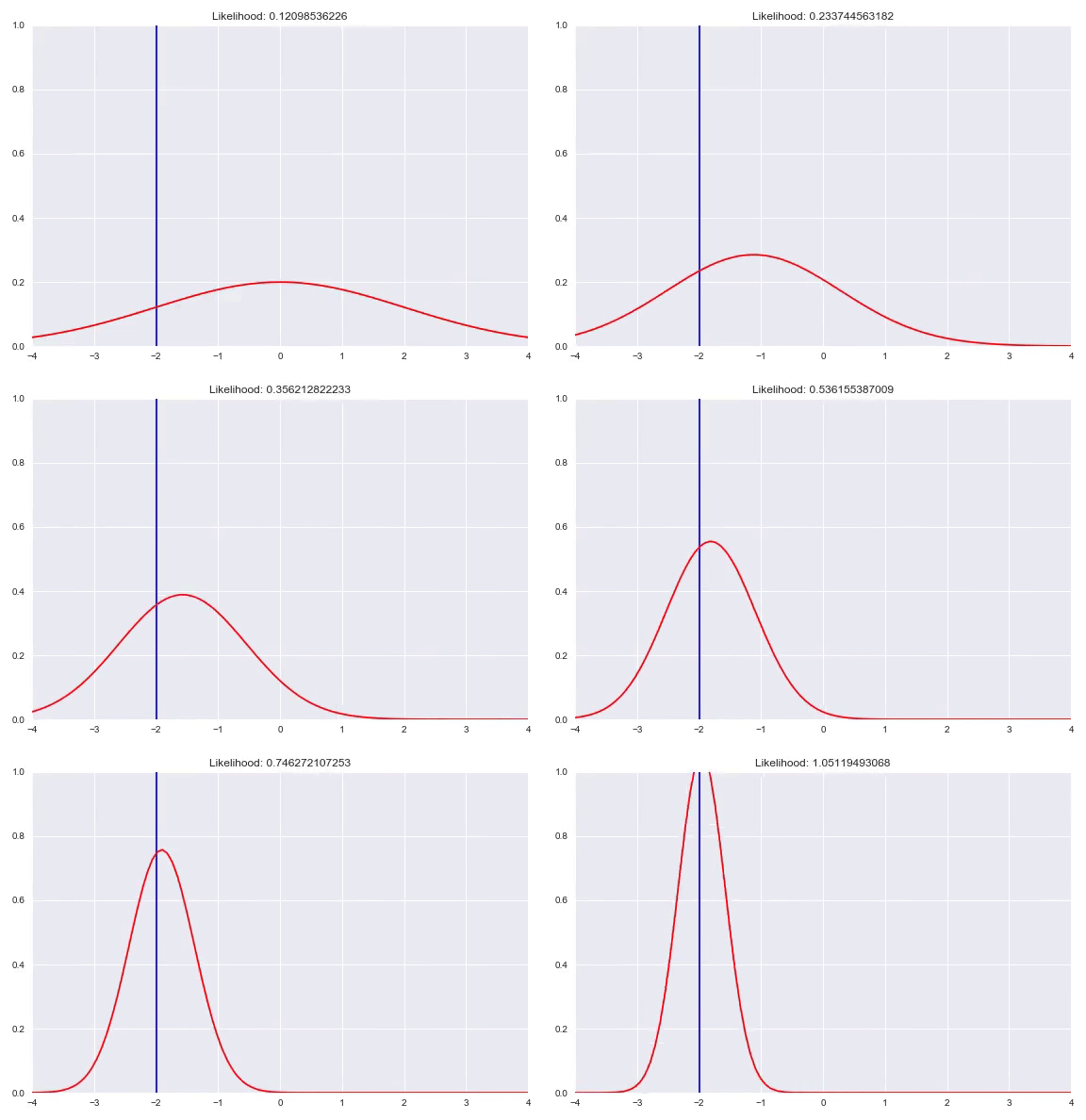
We can extend this idea by having a mixture of multiple distributions. In addition to the direct parameters of all the distributions, we also need to determine the weights for all the subdistributions similar to the quantized softmax approach. In the case of a mixture of k Gaussians we would have 3k parameters to estimate. k $\sigma$, which are again transformed to be strictly positive, k $\mu$ that are just a linear combination of the previous layer and k $\pi$, a softmax distribution over the different distributions. You can also use different distribution families in your mixture, however it is common practice to choose one, based on the range of your targets. Besides Gaussians, here are a few alternatives that you could use:

Beta distribution:

Support is $x\in \left[0,1\right]$ or $x\in \left(0,1\right)$

Parameters: $\alpha$ and $\beta$.

Density: $\frac{x^{\alpha-1}(1-x)^{\beta-1}}{B(\alpha,\beta)}$ with $B(\alpha,\beta)=\frac{\Gamma(\alpha)\Gamma(\beta)}{\Gamma(\alpha+\beta)}$.

Use case: modeling density over probabilities, fractions or other quantities in $\left[0,1\right]$.

Gamma distribution:

Support: $x\in \left(0,\infty\right)$.

It has two common parameterizations, we will use the Bayesian one with shape $\alpha$ and rate $\beta$.

Density: $\frac{\beta^\alpha}{\Gamma(\alpha)}x^{\alpha-1}e^{-\beta x}$

Use case: commonly used for approximating distributions over strictly positive values. Another option for this range could be the Weibull distribution.

Of course these distributions are easy to shift. Any parametric distribution that has a differentiable density function can be used in this way, however, be aware that training these density mixture networks can be difficult. Initialization can be tricky and sometimes has to be done again when the likelihood is $0$ for certain points. In that regard, make sure to normalize your targets to zero mean and unit variance, so that the expectation of your initialization is also $0$ (initialize all your biases at 0). Even when the initialization is working, sometimes the network will get in a part of the parameter space where one of your training samples will suddenly fall outside of a positive density and break your network.

Kernel Mixture Networks

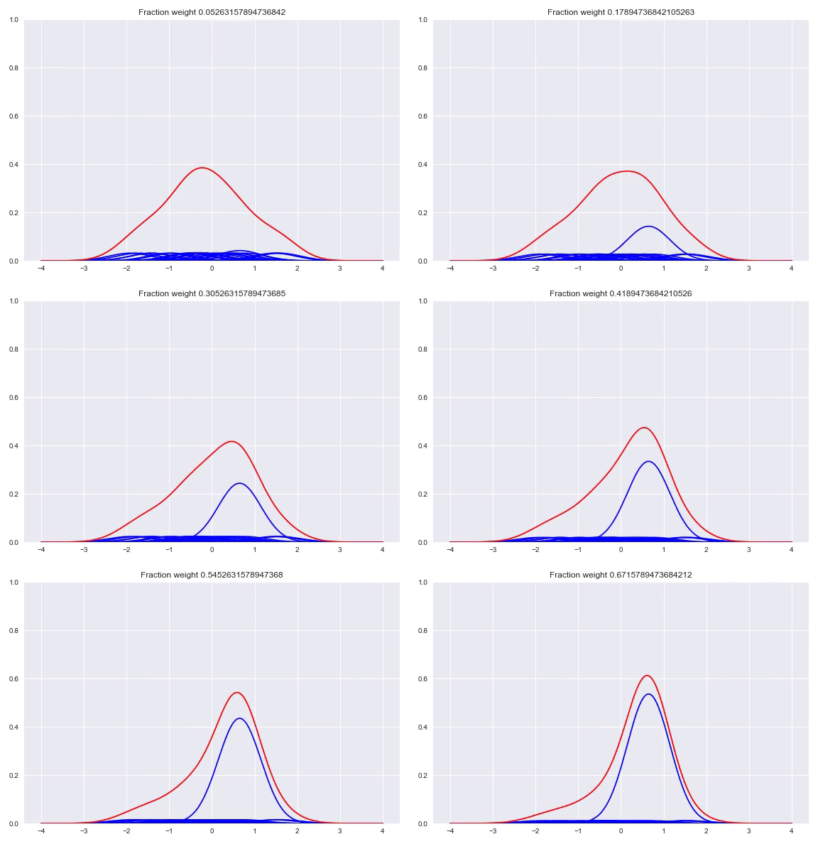
In the paper The Kernel Mixture Network: A Nonparametric Method for Conditional Density Estimation of Continuous Random Variables the authors combine the approach of unconditional kernel density and quantized softmax networks, in order to obtain a conditional kernel density. The idea is fairly simple, but elegant. Similar to unconditional kernel density estimation, we use all the targets of our training samples or a sampled subset as kernels for our distribution. However, instead of weighing each one of them uniformly, we want to redistribute the weight conditioned on our input. This approach is basically the same as quantized softmax networks, however, here we use kernel densities instead of discretized bins. In the following animation you can see all the weight slowly going towards one of the kernels:

The following happens when we move all the weights equally to two different kernels and arrive at a bimodal distribution:

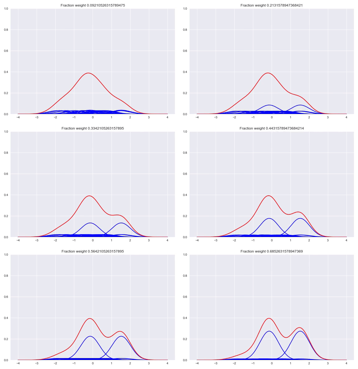
Like before, the output layer is a softmax layer which indicates the weight for each kernel. Conveniently, with this architecture the kernels itself don’t even need to be differentiable because we only adjust the weights of the kernels, the kernel value between the center and the point to be queried is consideren constant during training. First we will look at picking the kernels and bandwidths, followed by our implementation in TensorFlow, Edward + Keras and potential extensions of this method.

Kernels and bandwidths

The kernels form the bases for the densities. While the shape of the kernels might not be too relevant, the bandwidth determines a lot about the shape of the output density. If the bandwidth is too small, spikes show up in the densities that are typical of overfitting. Corresponding to this the evaluation likelihood will become poor because targets that are a bit further from the kernel centers will have a low likelihood. On the other hand, if your bandwidth is too wide you lose information, the distributions will have a very generic shape and your likelihood will be bad because the distributions is very unspecific. The bandwidth to use is a hyperparameter of the model, as it is described in the paper. We will get back to this later.

In small data scenarios using all the targets as kernel centers is a good strategy, however there will be diminishing returns with bigger data sets, due to highly similar targets. The network has no use for duplicate kernels while it does increase the degrees of freedom of the network and decrease performance. The paper removes a kernel center when it’s very close to another kernel center. Our suggestion is to use clustering on your target space instead, basically averaging centers that are close together. This idea is inspired by Radial Basis Function networks that were used in the past, they initialize their radial kernels in a similar fashion. There are other similarities between the approaches, the big difference is that RBF networks use these kernels as feature extractors while Kernel Mixture networks use the kernels to parameterize the output distribution. If you cluster to a high number of centers, another suggestion that we have not actually tested is to keep the edges as centers, because your model cannot express modes that are outside the centers on the edges, kind of reducing the range of your network if you throw away the edge cases. With a low number of centers this is probably not worth it. Our implementation includes the ‘use all’, ‘k-means’ and ‘agglomerative’ clustering approaches to get a list of kernel centers to use. In the case of 1-dimensional clustering, there is a better alternative for k-means like Jenks natural breaks optimization but we used k-means because it doesn’t matter too much and sci-kit learn has an easy API.

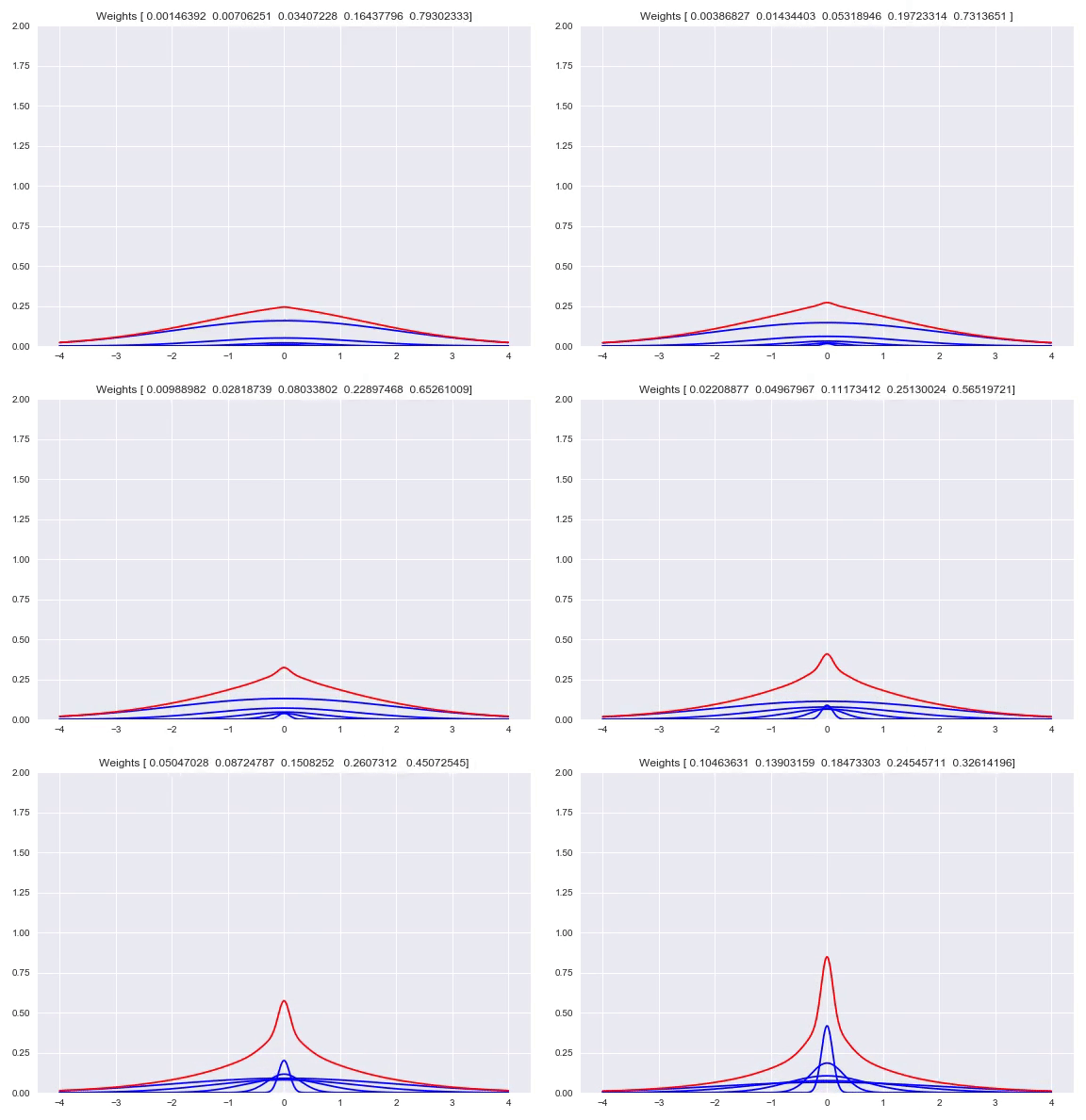
Using one bandwidth allows for small or wide distributions by putting all the weight in one kernel or spreading the weights over multiple kernels. Instead of having one bandwidth we could also have multiple kernels per center, each with their own bandwidth. This allows for adjusting the spread around one center, based on our input. Here you can see the effect of shifting the weights around one center:

Now we will diverge a bit from the paper. There is no strong reason to keep the $\sigma$ fixed. Using backpropagation in our networks, we can adjust not just the weights in our network that parameterize the weights over our kernels, but also adjust our $\sigma$. When $\sigma$ becomes too small, the likelihood will get poor because of samples that have a very small density because they are a bit too far from kernels while the likelihood will also be poor with a bandwidth that is too high, because the density of the kernels is too flat. This is something that a network can learn itself relatively easy. Doing this means that our kernels now have to be subdifferentiable. Extending this to multiple bandwidths does not work as well as we hoped. What we see is that the list of different $\sigma$ almost converges to the same value. We believe this is due to the fact that for a training batch, all the $\sigma$ will be pulled in the same direction. There are some ways to combat this problem, you could add a penalty term to your loss function that punishes low variance in your $\sigma$ vector which means the network is incentivized to have more different values. Another way is to have one trainable $\sigma$ and use for example $\left[\sigma, 2\sigma, 3\sigma, 4\sigma\right]$ as bandwidths. We have not tested these options yet but they are easy to implement.

Another thing to notice is that this concept is very natural to extend to multiple output dimensions. Instead of using 1-dimensional Gaussian kernels, we can also use n-dimensional Gaussian kernels, by using the squared norm between the $\mathbf{y}$ and $\mathbf{y}’$ output vectors. If we look at the uncorrelated multivariate Gaussian distribution, our Kernel function turns into:

Of course the output dimensions itself are not uncorrelated, but they both depend on the same latent representation that is learned by the network.

Implementation

We have implemented the paper and ideas in a class consiting of a combination of TensorFlow, Edward and Keras, where you can easily plugin your own network and data and add a Kernel Mixture Network output layer to output conditional distributions over your target. Here we will look at an implementation in TensorFlow which is a bit lower level, to get a better understanding of how it works. We will use k-means clustering from sci-kit learn for finding the centers and use Gaussian kernels with multiple, non-trainable bandwidths.

First we need to cluster the targets, here is an easy routine for ‘k-means:

import numpy as np
from sklearn.cluster import KMeans

def kmeans_centers(y, k=100):
    kmeans = KMeans(n_clusters=k, n_jobs=-2)
    kmeans.fit(np.array(train_y).reshape(-1, 1))
    cluster_centers = kmeans.cluster_centers_
    return cluster_centers.ravel()

Next, we need a Gaussian kernel function that calculates the kernel value between two values, during training this will be between the observed $y$ and kernel center $y^{(p)}$. This will be a TensorFlow node in our graph that outputs a new tensor. The kernel function is:

from math import pi
import tensorflow as tf

def gaussian_kernel(y, y_acc, sigma):
    return 1. / (tf.sqrt(2 * pi) * sigma * tf.exp(-tf.square(y - y_acc) / (2 * tf.square(sigma))

If the parameter $\sigma$ is a TensorFlow Variable instead of a constant this is instantly trainable. Now we want to define the final output layer that takes the weight tensor, the target $y$, a list of kernel centers and a $\sigma$ and that will return the density for the passed $y$, given the weights.

def density_output_layer(w, y, cluster_centers, sigma):
    output_kernels = []
    for center in cluster_centers:
        output_kernels.append(tf.reshape(gaussian_kernel(y, center, sigma), [-1, 1]))
    output_kernels = tf.concat(output_kernels, axis=1)
    output_nodes = tf.multiply(w, output_kernels)
    return tf.reduce_sum(output_nodes, axis=1) / total_weight

This layer takes in the second to last layer of the network which has a form of a softmax output to make sure the density still sums to one. If we pass a list of n constant $\sigma$ or a list of n trainable $\sigma$ variables, we can iterate over those within the center loop to have different bandwidths for every kernel center. If you do this you have to make sure to index the kernels correctly in case of sampling from the predicted output distribution.

After wiring the inputs, normal layers, the softmax weight layer and the density output layer together we can put in samples $x$ and a $y$ and the network returns the density of this specific $y$ given our input $x$. To train the network we need a loss function however, fortunately the negative log-likelihood is easy once we have access to the density. Here is the function:

In this case $n$ is the size of our training batch. If our density output layer is called ‘density’, our loss function is defined as follows:

loss = -tf.log(density)
mean_loss = tf.reduce_mean(loss)
train = tf.train.AdamOptimizer().minimize(mean_loss)

Once we have our train operation in our TensorFlow graph we can pass batches and optimize our network. If we want to sample from a conditional distribution, we can first sample from our weights output which is a discrete probability distribution, and then from the corresponding kernel. Our class made using Edward has a clean sampling method baked in.

Plug and play class

We worked on a basic class that you can use to build Kernel Mixture Networks. You can plug in your own base estimator made in TensorFlow or Keras and fit it to your data. While it is not very extensive it should be easy to extend it with allowing lists of input placeholders or using different kernels or center strategies. Here we will go over a quick example using a toy dataset from the Edward website:

def build_toy_dataset(nsample=40000):
    y_data = np.float32(np.random.uniform(-10.5, 10.5, (1, nsample))).T
    r_data = np.float32(np.random.normal(size=(nsample,1))) # random noise
    x_data = np.float32(np.sin(0.75*y_data)*7.0+y_data*0.5+r_data*1.0)
    X_train, X_test, y_train, y_test = train_test_split(x_data, y_data, random_state=42, train_size=0.5)
    return X_train, X_test, y_train.ravel(), y_test.ravel()

X_train, X_test, y_train, y_test = build_toy_dataset(40000)

sns.regplot(X_train, y_train, fit_reg=False)

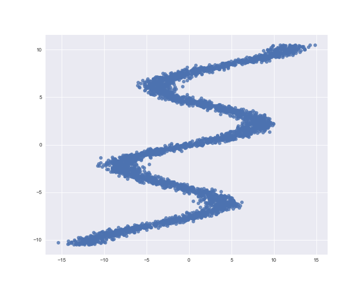
Let’s build a normal, feed forward network in Keras as the start of our Kernel Mixture network, next to our customer class, all we need are a placeholder from TensorFlow and the Dense layer from Keras.

from src.kmn import KernelMixtureNetwork
from keras.layers import Dense
import tensorflow as tf

X_ph = tf.placeholder(tf.float32, [None, 1])
model = Dense(32, activation='relu')(X_ph)
model = Dense(16, activation='relu')(model)
model = KernelMixtureNetwork(estimator=model, X_ph=X_ph, train_scales=True)
kmn.fit(X_train, y_train, n_epoch=300, eval_set=(X_test, y_test))

We can plot our loss curves via .plot_loss()

kmn.plot_loss()

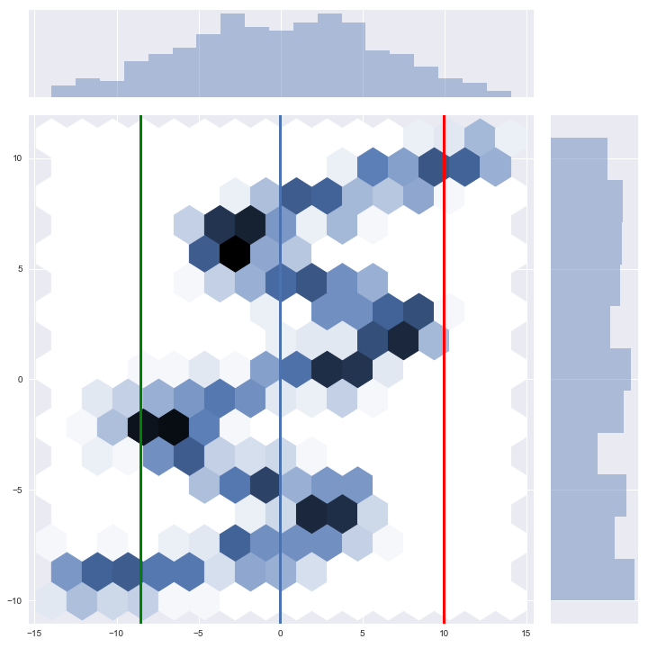
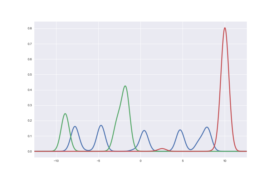
Now we can sample from the network conditioned on the $x$ values in our test set and look at the density in total, and zoom in on a few examples (they are the vertical, colored lines).

samples = model.sample(X_test)
jp = sns.jointplot(X_test.ravel(), samples, kind="hex", stat_func=None, size=10)
jp.ax_joint.add_line(Line2D([X_test[0][0], X_test[0][0]], [-40, 40], linewidth=3))
jp.ax_joint.add_line(Line2D([X_test[1][0], X_test[1][0]], [-40, 40], color='g', linewidth=3))
jp.ax_joint.add_line(Line2D([X_test[2][0], X_test[2][0]], [-40, 40], color='r', linewidth=3))

As we can see here, the total population of our samples certainly resembles our input. The conditional density of the first three samples also fit very well:

d = model.predict_density(X_test[0:3,:].reshape(-1,1), resolution=1000)
df = pd.DataFrame(d).transpose()
df.index = np.linspace(kmn.y_min, kmn.y_max, num=1000)
df.plot(legend=False, linewidth=3, figsize=(12.2, 8))

Make sure to check out the notebook where all of the previous code is gathered.

Conclusion

First we looked at some ways to describe distributions and extended this into conditioning those distributions using neural networks. Next to the advantages and disadvantages of different methods, we also dove into an implementation of Mixture Density Networks. In my opinion it’s a very clean way of solving this problem. I do believe there are some additional tricks available to get better performance like toying around more with the trainable bandwidths, mixing different kernels similar to mixing multiple bandwidths or different kernel center initialization. The nice thing about this method is that it appear very numerically stable and that you can put it on top of any part of a neural network graph that outputs a single vector given an input, which means this goes on top of CNNs and LSTMs just as well as on normal architectures.

I learned a lot during this small project and I hope you did as well by reading my first blog post. I would be happy to get feedback on the content and on the structure of this post, because I already have a few other topics scheduled. Thank you for reading!